What is ClickHouse?
ClickHouse® is a high-performance, column-oriented SQL database management system (DBMS) for online analytical processing (OLAP). It is available as both an open-source software and a cloud offering.
What is OLAP?
OLAP scenarios require real-time responses on top of large datasets for complex analytical queries with the following characteristics:
- Datasets can be massive - billions or trillions of rows
- Data is organized in tables that contain many columns
- Only a few columns are selected to answer any particular query
- Results must be returned in milliseconds or seconds
Column-Oriented vs Row-Oriented Databases
In a row-oriented DBMS, data is stored in rows, with all the values related to a row physically stored next to each other.
In a column-oriented DBMS, data is stored in columns, with values from the same columns stored together.
Why Column-Oriented Databases Work Better in the OLAP Scenario
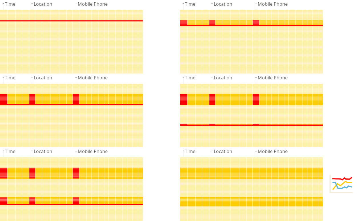
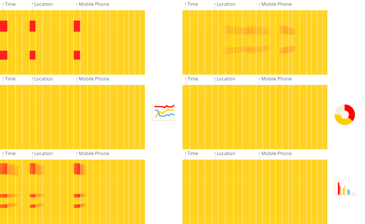
Column-oriented databases are better suited to OLAP scenarios: they are at least 100 times faster in processing most queries. The reasons are explained in detail below, but the fact is easier to demonstrate visually:
Row-oriented DBMS

Column-oriented DBMS

See the difference?
The rest of this article explains why column-oriented databases work well for these scenarios, and why ClickHouse in particular outperforms others in this category.
Why is ClickHouse so fast?
ClickHouse uses all available system resources to their full potential to process each analytical query as fast as possible. This is made possible due to a unique combination of analytical capabilities and attention to the low-level details required to implement the fastest OLAP database.
Helpful articles to dive deeper into this topic include:
Processing Analytical Queries in Real Time
In a row-oriented DBMS, data is stored in this order:
| Row | WatchID | JavaEnable | Title | GoodEvent | EventTime |
|---|---|---|---|---|---|
| #0 | 89354350662 | 1 | Investor Relations | 1 | 2016-05-18 05:19:20 |
| #1 | 90329509958 | 0 | Contact us | 1 | 2016-05-18 08:10:20 |
| #2 | 89953706054 | 1 | Mission | 1 | 2016-05-18 07:38:00 |
| #N | … | … | … | … | … |
In other words, all the values related to a row are physically stored next to each other.
Examples of a row-oriented DBMS are MySQL, Postgres, and MS SQL Server.
In a column-oriented DBMS, data is stored like this:
| Row: | #0 | #1 | #2 | #N |
|---|---|---|---|---|
| WatchID: | 89354350662 | 90329509958 | 89953706054 | … |
| JavaEnable: | 1 | 0 | 1 | … |
| Title: | Investor Relations | Contact us | Mission | … |
| GoodEvent: | 1 | 1 | 1 | … |
| EventTime: | 2016-05-18 05:19:20 | 2016-05-18 08:10:20 | 2016-05-18 07:38:00 | … |
These examples only show the order that data is arranged in. The values from different columns are stored separately, and data from the same column is stored together.
Examples of a column-oriented DBMS: Vertica, Paraccel (Actian Matrix and Amazon Redshift), Sybase IQ, Exasol, Infobright, InfiniDB, MonetDB (VectorWise and Actian Vector), LucidDB, SAP HANA, Google Dremel, Google PowerDrill, Druid, and kdb+.
Different orders for storing data are better suited to different scenarios. The data access scenario refers to what queries are made, how often, and in what proportion; how much data is read for each type of query – rows, columns, and bytes; the relationship between reading and updating data; the working size of the data and how locally it is used; whether transactions are used, and how isolated they are; requirements for data replication and logical integrity; requirements for latency and throughput for each type of query, and so on.
The higher the load on the system, the more important it is to customize the system set up to match the requirements of the usage scenario, and the more fine grained this customization becomes. There is no system that is equally well-suited to significantly different scenarios. If a system is adaptable to a wide set of scenarios, under a high load, the system will handle all the scenarios equally poorly, or will work well for just one or few of possible scenarios.
Key Properties of OLAP Scenario
- Tables are “wide,” meaning they contain a large number of columns.
- Datasets are large and queries require high throughput when processing a single query (up to billions of rows per second per server).
- Column values are fairly small: numbers and short strings (for example, 60 bytes per URL).
- Queries extract a large number of rows, but only a small subset of columns.
- For simple queries, latencies around 50ms are allowed.
- There is one large table per query; all tables are small, except for one.
- A query result is significantly smaller than the source data. In other words, data is filtered or aggregated, so the result fits in a single server’s RAM.
- Queries are relatively rare (usually hundreds of queries per server or less per second).
- Inserts happen in fairly large batches (> 1000 rows), not by single rows.
- Transactions are not necessary.
It is easy to see that the OLAP scenario is very different from other popular scenarios (such as OLTP or Key-Value access). So it does not make sense to try to use OLTP or a Key-Value DB for processing analytical queries if you want to get decent performance. For example, if you try to use MongoDB or Redis for analytics, you will get very poor performance compared to OLAP databases.
Input/output
- For an analytical query, only a small number of table columns need to be read. In a column-oriented database, you can read just the data you need. For example, if you need 5 columns out of 100, you can expect a 20-fold reduction in I/O.
- Since data is read in packets, it is easier to compress. Data in columns is also easier to compress. This further reduces the I/O volume.
- Due to the reduced I/O, more data fits in the system cache.
For example, the query “count the number of records for each advertising platform” requires reading one “advertising platform ID” column, which takes up 1 byte uncompressed. If most of the traffic was not from advertising platforms, you can expect at least 10-fold compression of this column. When using a quick compression algorithm, data decompression is possible at a speed of at least several gigabytes of uncompressed data per second. In other words, this query can be processed at a speed of approximately several billion rows per second on a single server. This speed is actually achieved in practice.
CPU
Since executing a query requires processing a large number of rows, it helps to dispatch all operations for entire vectors instead of for separate rows, or to implement the query engine so that there is almost no dispatching cost. If you do not do this, with any half-decent disk subsystem, the query interpreter inevitably stalls the CPU. It makes sense to both store data in columns and process it, when possible, by columns.
There are two ways to do this:
A vector engine. All operations are written for vectors, instead of for separate values. This means you do not need to call operations very often, and dispatching costs are negligible. Operation code contains an optimized internal cycle.
Code generation. The code generated for the query has all the indirect calls in it.
This is not done in row-oriented databases, because it does not make sense when running simple queries. However, there are exceptions. For example, MemSQL uses code generation to reduce latency when processing SQL queries. (For comparison, analytical DBMSs require optimization of throughput, not latency.)
Note that for CPU efficiency, the query language must be declarative (SQL or MDX), or at least a vector (J, K). The query should only contain implicit loops, allowing for optimization.